Calculating Seawater Chemistry Parameters
methods sws 15 Sep 2023Overview
Carbonate chemistry and dissolved oxygen are important parameters that capture the main processes occuring on coral reefs, including net productivity and net calcification. We will learn how to measure and calculate a suite of parameters that impact coral growth and health and characterize climate change.
General Background
Dissolved Oxygen
Dissolved oxygen (DO) is the amount of oxygen in seawater directly available to living organisms and is normally altered by the balance of photosynthesis and respiration of all community constituents. DO is traditionally expressed in units of O2 mg/L, % Air saturation, kPa, or $\mu$mol O2/L. When characterizing reef environments, these four units are interchangeable. kPa and % Air saturation are dependent upon temperature, salinity, and depth, while the other units are pressure-free quantities. By convention, coral incubations generally use $\mu$mol O2/L.
Hypoxia, or insufficient availability of DO, is defined as DO < 2mg/L (29% Air saturation/ 6 kPa / 63 $\mu$mol O2/L). Low oxygen, but not hypoxia, is defined as DO < 5 mg/L (73% Air saturation/ 15 kPa / 156 $\mu$mol O2/L). Hypoxia or low oxygen can be induced by warming, restricted water flow, increased biological oxygen demand, nutrient and organic matter loading, or influx of oxygen poor water.
Normoxic reefs, or the oxygen conditions normally experienced in healthy reef environments, have a mean daily DO of 5.7 mg/L (88% Air saturation/ 18.3 kPa / 173 $\mu$mol O2/L), mean daily range of 2.6 mg/L (42% Air saturation/ 8.6 kPa / 81 $\mu$mol O2/L ), a mean daily minimum of 4.4 mg/L (69% Air saturation/ 14.5 kPa / 137 $\mu$mol O2/L), and a mean daily maximum of 7.1 mg/L (111% Air saturation/ 22.9 kPa / 217 $\mu$mol O2/L). These mean normoxia values come from autonomous sensor data aggregated by Pezner AK et al. (2023) Nat Clim Chang. 13:403-409, and provide a general overview of present-day oxygen conditions. Reef DO will vary as a function of benthic community composition, where higher scleractinian coral cover will have higher daily maximums compared to an algal dominated reef due to the high rates of endosymbiont photosynthesis.
Dissolved oxygen concentrations can be measured amperometricly on discrete water samples with the Winkler Titration or with oxygen optodes which leverage photo quenching of oxygen sensitive compounds. Generally, amperometric measurements are considered the most accurate, while optodes permit long term monitoring with in-situ autonomous sensors or continuous monitoring of incubation chambers. We will use both methods in this course. For details on the Winkler Titration, please refer to Langdon (2010) “Determination of Dissolved Oxygen in Seaweater By Winkler Titration using Amperometric Technique.”
Since DO is a dynamic measurement which changes throughout the day, it is imperative that discrete water samples are collected at approximately the same time to minimize variability in the collected water samples.
Carbonate Chemistry
Ultimately, a “healthy” coral reef is defined by its ability to grow faster than dissolution and erosion processes since all ecological functions and ecosystem services are dependent upon the persistence of the physical reef structure. Growth is predominantly the result of continuous deposition of aragonite by hermatypic or reef building corals. Corals, and “healthy” reefs, therefore, need water chemistry that is favorable for calcification.
Coral calcification proceeds according to, $Ca^{2+} + CO_3^{2-} \iff CaCO_3$, where calcium and carbonate ions are combined within the coral tissues to build the aragonite coral skeleton. One can quantify the thermodynamics of calcium carbonate formation by looking at the aragonite or calcite saturation state ($\Omega$), which measures supersaturation of the respective mineral in a body of water. You can measure saturation state as $\Omega = \frac{[Ca^{2+}][CO_3^{2-}]}{K_{sp}}$, where $K_{sp}$ is the solubility of aragonite or calcite. When $\Omega < 1$, dissolution is thermodynamically favorable; when $1 < \Omega < 4$, calcifying proceeds at a low rate with mineralogical conformations; when $\Omega > 4$, calcification is thermodynamically favorable and reef growth generally persists.
The dominant driver of $\Omega$ is the net change in $[CO_3^{2-}]$. Under ocean acidification scenarios, carbonate ions react with carbon dioxide to form bicarbonate. Thus, $[HCO_3^-]$ increases and $[CO_3^{2-}]$ decreases, reducing the calcium carbonate saturation state. Conversely, under alkalinity enhancement, the equilibrium switches and the equation reverses, where bicarbonate breaks down to increase $[CO_3^{2-}]$, thereby increasing the calcium carbonate saturation state.
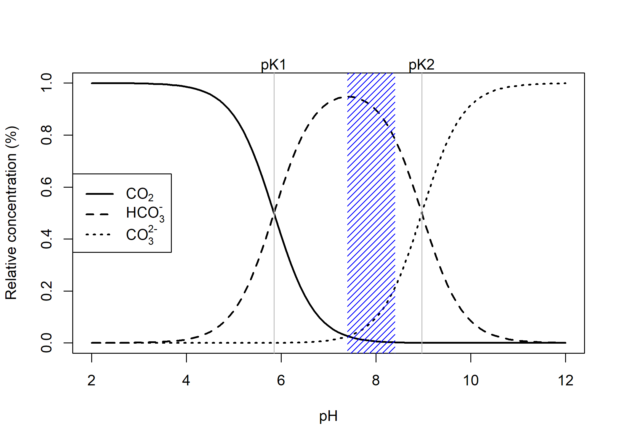
Dissolved inorganic carbon (DIC) is the total pool of inorganic carbon species in seawater, which includes carbonate, bicarbonate, and carbon dioxide. Under ocean acidification, DIC increases due to the oceanic uptake of carbon dioxide. The fraction of DIC species is pH dependent and can be readily visualized as follows,
Figure 1. DIC speciation plot, shaded region corresponds to reef pH under extreme OA to historical pH values
Total Alkalinity (TA, sometimes stylized in papers as $A_T$) can be defined as the total buffering capacity of seawater, or the excess of proton receptors over proton donors,
TA is influenced predominantly by bicarbonate and carbonate ion concentration along with a myriad of other minor constituents (Dickson AG 1981).
The three main processes on coral reefs, calcification, photosynthesis, and respiration, are collectively referred to as the reef metabolism. Calcification releases two protons for every mole of calcium carbonate precipitated, and therefore will alter total alkalinity in a 2:1 ratio of $\Delta$TA : calcification. Photosynthesis and respiration alter DIC, due to changes in CO2, but do not change TA. Therefore, you can describe metabolic processes (calcification/photosynthesis), by knowing both DIC and TA. This is known as measuring the metabolic pulse of coral reefs and must be done on discrete water samples (Cyronak T et al. 2018). Ongoing research seeks to characterize these metabolic processes from autonomous sensors, which measure DO and pH alone (Cryer SE et al. 2023.). While, DO and pH are related to DIC and TA, the relationships aren’t perfectly 1:1, and therefore, assumptions and limitations must be clearly defined. Nevertheless, this science presents a means to scale coral reef biogeochemistry research across space and time to better understand temporal dynamics and reef degradation under climate change.
Since carbonate chemistry is dynamic similar to DO, it is imperative that discrete water samples are collected at approximately the same time to minimize variability in the collected water samples.
Analytical Water Chemistry
We will go over each instrument and its SOP in detail. The following section details how to work with the measured data.
Carbonate Chemsitry
Hopefully from the section above, you begin to see that there is slight overlap among each of these measurements. In fact there are four total parameters, all of which are thermodynamically constrained by each other. Therefore, as long as you measure two parameters, you can calculate the complete carbonate chemistry suite. Generally you measure DIC and TA or pH and TA, as well as pressure related parameters including temperature, salinity, and depth. In our class, we will measure TA and pH to calculate all other parameters.
Seacarb
You can get into the weeds with the chemistry if you’d like. But as long as you understand everything thus far, you’re all set. We will use the seacarb package developed by biogeochemist Jean-Pierre Gattuso. This has largely replaced CO2SYS, which has been at the forefront of carbonate chemistry calculations for over 25 years. You may find reference to CO2SYS in the literature, just understand it does the same thing as seacarb.
Within the seacarb package, we will mostly use the carb function with flag=8 (where we supply pH and TA, respectively) and additionally supply the salinity and temperature we recorded when the seawater sample was collected. The defaults for other arguments follow the Guide to best practices for ocean CO2 measurements, so we do not need to mess with them. We measure TA in $\mu$mol/kg, but seacarb wants TA in mol/kg, so make sure to divide var2 by 1,000,000.
install.packages("seacarb")

carb(flag = 8, #which two variables are you supplying? we will use 8 (pH,TA)
     #variable values in the respective order, units must be mol/kg except for pH
     var1 = pH, var2 = TA.umol_kg/1000000,
     # salinity and temperature of the in situ conditions
     S = sal, T = temp)
Other useful functions include pHconv to convert from total, seawater, and free scale and pHinsi to temperature correct pH if it was spectrophotometrically measured at a different temperature than when it was collected. As always, run ?pHconv or any other function in R to see the documentation, which will help you better understand the function.
Dissolved Oxygen
We will use dissolved oxygen data both to calculate the average conditions the corals were exposed to and to manipulate incubation data to calculate productivity rates.
respR
The respR package has many helpful functions to automatically analyze respirometry data. Its most helpful function is convert_DO() to convert between different units of DO including O2 mg/L, % air saturation, or $\mu$mol O2/L.
I used the above equation to build the following table,
Table 1. DO unit equivalencies at 25, 30, and 35 C and S=35ppt
|
% Air saturation
|
|||||
|---|---|---|---|---|---|
| S | mg/L | umol/L | 25 | 30 | 35 |
| 35 | 1.50 | 46.87676 | 22.21860 | 24.11961 | 26.04365 |
| 35 | 2.25 | 70.31514 | 33.32789 | 36.17941 | 39.06548 |
| 35 | 3.50 | 109.37910 | 51.84339 | 56.27908 | 60.76852 |
| 35 | 4.50 | 140.63027 | 66.65579 | 72.35882 | 78.13095 |
| 35 | 4.75 | 148.44307 | 70.35889 | 76.37876 | 82.47156 |
| 35 | 5.75 | 179.69424 | 85.17128 | 92.45849 | 99.83399 |
| 35 | 6.00 | 187.50703 | 88.87438 | 96.47843 | 104.17460 |
| 35 | 6.75 | 210.94541 | 99.98368 | 108.53823 | 117.19643 |
| 35 | 8.00 | 250.00938 | 118.49917 | 128.63791 | 138.89947 |
| 35 | 8.75 | 273.44775 | 129.60847 | 140.69771 | 151.92129 |
Analyzing Respirometry Data
Figure 2. Example Respirometry Data Analysis
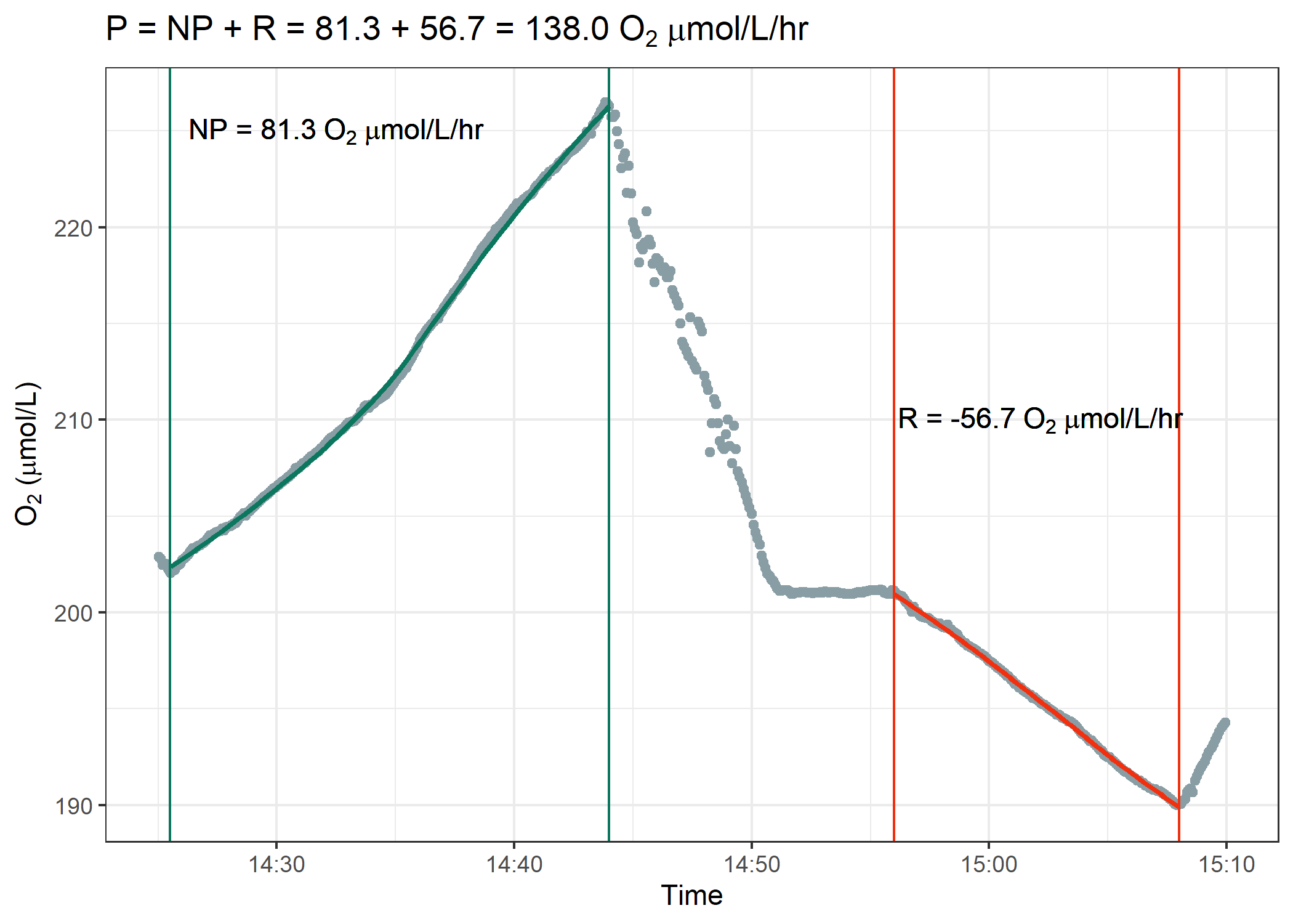
The goal is to analyze the respirometry data identical to the figure above. You first need to identify the region where we measured net photosynthesis and then the second region where we measured respiration. Over each discrete region, calculate a linear regression and extract the slope. This slope will be in units of $\mu$mol $O_2$ / L / minute. Multiply this rate by 60 since we want respiration and net photosynthesis values in rates per hour. Finally, add the absolute value of respiration to net photosynthesis to determine gross photosynthesis rates.
The most efficient way to analyze all this data at once is to add case_when statements to the respirometry data and define the measurement type (“NP” or “R”) based on the metadata, which indicates when each incubation started and ended. You will want to use the between function for this. Then, nest the data to create individual data frames for each incubation type for each coral, which we define by the unique coral ID. See code example below:
respirometry_data %>%
  # combine Date and Time into one column
  mutate(datetime = mdy_hms(paste(Date,Time))) %>%
  # encode manually
  # build a bunch of conditional statements to pinpoint a incubation
                          # chamber 1, net photosynthesis start/stop
  mutate(type = case_when(chamber == 1 & between(datetime,
                                         ymd_hms("2023-09-15 14:56:00 UTC"),
                                         ymd_hms("2023-09-15 15:08:00 UTC")) ~ "NP",
                          # chamber 1, respiration start/stop
                          chamber == 1 & between(datetime,
                                         ymd_hms("2023-09-15 15:14:00 UTC"),
                                         ymd_hms("2023-09-15 15:25:00 UTC")) ~ "R",
                          # do this for all chamber and start/stop times
                          TRUE ~ NA),
                            # chamber 1, NP start through R end
         coralID = case_when(chamber == 1 & between(datetime,
                                        ymd_hms("2023-09-15 14:56:00 UTC"),
                                        ymd_hms("2023-09-15 15:25:00 UTC")) ~ 123,
                          # do this for all chamber and start/stop times
                          TRUE ~ NA)) %>%
  group_by(chamber) %>%
   # need to linearly correct oxygen since calibration was wonky
 mutate(baseLine = subset(.,row_number()<=5) %>% pull(O2) %>% mean(),
        O2 = O2*(1+(202.6-baseLine)/baseLine)) %>%
  ungroup() %>%
  # remove data when not inside a incubation
  drop_na(type,coralID) %>%
  group_by(coralID, type) %>%
  # create minute column
  mutate(min = as.numeric(datetime - first(datetime))/60)
    select(-baseLine)) %>%
  # nest individual incubations within coralID/type definitions
  nest() %>%
  # create a linear model for each incubation, extract the slope
  mutate(fit   = map(data, ~lm(O2 ~ datetime, data = .)),
         slope = map(fit, function(df) (tidy(df) %>% pull(estimate))[2]*60)) %>%
  # unnest the slope
  unnest(slope) %>%
  # move the NP,R incubations into their own column for each coralID
  pivot_wider(names_from = "type",
              values_from = "slope") %>%
  # keep only coralID, R/NP slope (add other cols you want to keep if desired)
  select(coralID, R, NP) %>%
  # calculate P from NP, R
  mutate(P = NP + abs(R))
You can likely achieve the same results without all the case_when statements by left_join the metadata table based on chamber number and times and then use the fill verb to copy the metadata to multiple corresponding rows. But that code would take a bit more time to figure out. If you’d like to learn how we’d go about this method, we can work on it together.