Organizing Spec Hypoxia Data
methods sws 06 Sep 2023Overview
Anaerobic respiration pathways are diverse and predate the evolution of photosynthesis. With the predicted increase in hypoxia events on coral reefs, it is imperative that scientists understand coral metabolism in low-oxygen environments to better predict coral health and survival under future climate change scenarios. There are four conserved pathways among eukaryotes we will be investigating within our coral hypoxia experiment, including lactate (LDH), octopine (ODH), alanopine (ADH), and strombine (SDH) dehydrogenase activities, all of which oxidize NADH during anaerobic respiration. You can read more about these enzymes and their roles in coral metabolism by reading, Murphy and Richmond (2016) doi:10.7717/peerj.1956 and the references within, or consult your Cellular and Molecular Biology textbook.
The following sections detail how we quantitatively assess the activities of these four enzymes within corals. Briefly, we sample polyps from a coral, homogenize in a Tris buffer solution, aliquot to a 96-well plate with reagents, and measure the absorbance over time to calculate enzyme NADH oxidation activity. We will also measure total protein concentrations to standardize enzyme activity rates.
Load the Plate Map
A 96-well plate helps us efficiently analyze multiple samples and replicates of each sample. Because there are a lot of samples, however, it is easy to mixup which well corresponds to which coral. To solve this problem, we will use a plate map.
Table 1. Example of a 96-well plate map
| row | 1 | 2 | 3 | 4 | 5 | 6 | 7 | 8 | 9 | 10 | 11 | 12 |
|---|---|---|---|---|---|---|---|---|---|---|---|---|
| A | Sample1 | Sample1 | Sample1 | Sample2 | Sample2 | Sample2 | Sample3 | Sample3 | Sample3 | Sample4 | Sample4 | Sample4 |
| B | Sample5 | … | … | … | … | … | … | … | … | … | … | … |
| C | … | … | … | … | … | … | … | … | … | … | … | … |
| D | … | … | … | … | … | … | … | … | … | … | … | … |
| E | … | … | … | … | … | … | … | … | … | … | … | … |
| F | … | … | … | … | … | … | … | … | … | … | … | … |
| G | … | … | … | … | … | … | … | … | … | … | … | … |
| H | … | … | … | … | … | … | … | … | … | … | … | … |
It is important to follow the plate map carefully to keep track of samples and to later analyze the data with a script to automatically process the samples. You can find a copy of the plate map here.
For this format, keep in mind the following:
- The date should be in the first column in mm/dd/YYYY format, directly above the plates
- In column N, list all plate names that correspond with the map; one plate name per row
- Leave at least one blank row between distinct plate maps
- You can have multiple plates for one date and you can have multiple dates per excel file.
Plate Map Processing Code
# make sure the plate maps are in a folder all by themselves
map_files <- list.files("~/Grad School/TA/SWS-F23/data/templates/plateMaps/",
                        full.names = T)

# function to process 1 or more plate map files
plate_map <- lapply(map_files, function(x) {
  read_excel(x,
             col_names = c("row", 1:12, "plate_name")) %>%
# add the date as a column to each plate
  mutate(date = as.Date(as.numeric(row),
                        origin="1899-12-30"),
         .before = "row") %>%
    fill(date, .direction = "down")}) %>%
  bind_rows()

# grab the plate names
plate_names <- plate_map %>%
  select(date, plate_name) %>%
  drop_na() %>%
  # remove rows that have comments, delineated by an * in the plate name col
  filter(!str_detect(plate_name, '^\\*')) %>%
  mutate(plate_name = str_replace(plate_name,
                                     '(plate)|(PLATE)',
                                     ' '),
         # strip white space from names
         plate_name =str_replace_all(plate_name,
                                     "(\\S)\\s{2,}(?=\\S)", "\\1 "),
         # grab the plate type
         type = str_trim(str_extract(plate_name, "^.*(?=[[:digit:]])")))

plate_map <- plate_map %>%
  # remove the date row numeric
  filter(str_detect(row, "^[:alpha:]+$")) %>%
  # remove rows that correspond to an empty row on the plate
  filter(if_any(as.character(1:12),
                ~ !is.na(.))) %>%
  select(-plate_name) %>%
  #cast into long format
  pivot_longer(cols=as.character(1:12),
               names_to = "plate_map",
               values_to= "sample",
               values_drop_na = T) %>%
  mutate(plate_map = paste0(row,plate_map)) %>%
  select(-row)


#add plate num based on repeat value within a given date
plate_map <- plate_map %>%
  group_by(date, plate_map) %>%
  mutate(plate_num = row_number()) %>%
  ungroup() %>%
  left_join(plate_names %>%
              mutate(plate_num = as.integer(str_extract(plate_name,
                                                        "(\\d)+")))) %>%
  select(-plate_num)
Table 2. Processed plate map
| date | plate_map | sample | plate_name | type |
|---|---|---|---|---|
| 2023-08-25 | A1 | A1 | TAC 1 | TAC |
| 2023-08-25 | A1 | A1 | PROTEIN 1 | PROTEIN |
| 2023-08-25 | A2 | A1 | TAC 1 | TAC |
| 2023-08-25 | A2 | A1 | PROTEIN 1 | PROTEIN |
| 2023-08-25 | A3 | A1 | TAC 1 | TAC |
Load spectrophotometric data
The plate is then read on the plate spectrophotometer. Follow the protocols for incubation temperature, shake settings, read wavelength, and time. Ensure the naming scheme from the plate map is reproduced in the spectrophotometer computer so the saved file has identical names.
Common naming schemes include, “LDH 1 T18” for LDH plate 1 measured at the 18th minute, or “protein 2” for protein plate 2, or “TAC 1 initial” for the initial reading of TAC plate 1.
Spectrophotometric Data Processing Code
# make sure the spec files are in a folder all by themselves
spec_files <- list.files("~/Grad School/TA/SWS-F23/data/templates/spec/",
                         full.names = T)

spec_dat <- lapply(spec_files, function(x) {
  read.csv(file(x,
              encoding="UCS-2LE"),
         sep = "\t", header = F,skip = 1)[,1:14] %>%
  set_names(c("date","plate_name", 1:12)) %>%
  mutate(across(3:14, ~ as.numeric(.x))) %>%
  mutate(date = as.Date(str_extract(last(date),
                            "[[:digit:]]{1,2}\\/[[:digit:]]{1,2}\\/[[:digit:]]{4}"),
                        "%m/%d/%Y")) %>%
  #remove the unimportant rows
  filter(plate_name != 'Temperature(¡C)' | is.na(plate_name)) %>%
  #grab the correct plate name for each row
  mutate(plate_name = case_when(is.na(as.numeric(plate_name)) ~ plate_name,
                                TRUE ~ NA),
         # pull out the time point in its own col
         time = toupper(str_extract(plate_name,
                                    "(?<=[[:digit:]] ).*$")),
         # remove time point from plate name
         plate_name = str_trim(str_extract(plate_name,
                                           "^.* [[:digit:]]*(?=.*)"))) %>%
  fill(c(plate_name,time)) %>%
  #remove empty plate rows
  filter(if_any(as.character(1:12), ~ !is.na(.))) %>%
  group_by(plate_name, time) %>%
  #remove the metadata for the plate
  filter(row_number()!=1) %>%
  #append the row letter scheme
  mutate(row = case_when(row_number() == 1 ~ "A",
                         row_number() == 2 ~ "B",
                         row_number() == 3 ~ "C",
                         row_number() == 4 ~ "D",
                         row_number() == 5 ~ "E",
                         row_number() == 6 ~ "F",
                         row_number() == 7 ~ "G",
                         row_number() == 8 ~ "H",
                         TRUE ~ NA),
         .after="plate_name") %>%
  ungroup() %>%
  #build plate map from row and col
  pivot_longer(as.character(1:12),
               names_to = 'plate_map',
               values_to = 'Abs') %>%
  mutate(plate_map = paste0(row,plate_map)) %>%
  select(-row)
}) %>% bind_rows()
Table 3. Organized spectrophotometer data
| date | plate_name | time | plate_map | Abs |
|---|---|---|---|---|
| 2023-08-31 | LDH 1 | T0 | A1 | 0.0771 |
| 2023-08-31 | LDH 1 | T0 | A2 | 0.0736 |
| 2023-08-31 | LDH 1 | T0 | A3 | 0.0766 |
| 2023-08-31 | LDH 1 | T0 | A4 | 0.0767 |
| 2023-08-31 | LDH 1 | T0 | A5 | 0.0786 |
Process data
Now that you have your plate map and the raw spectrophotometric data organized, it’s time to join these data together and then analyze them.
First, join the plates together by common plate map well identifiers, plate name, and date the plate was analyzed. Then we will group together our triplicate measurements and take the average reading to be our accepted absorbance, which we will use for all future calculations.
dat <- spec_dat %>%
  #ignore the case sensitivity of the plate_name
  mutate(plate_name = toupper(plate_name)) %>%
  left_join(plate_map %>% mutate(plate_name = toupper(plate_name)),
            by = c("plate_map", "plate_name", "date")) %>%
  group_by(sample, type, time) %>%
  summarise(sd = sd(Abs, na.rm=T),
            Abs = mean(Abs, na.rm=T))
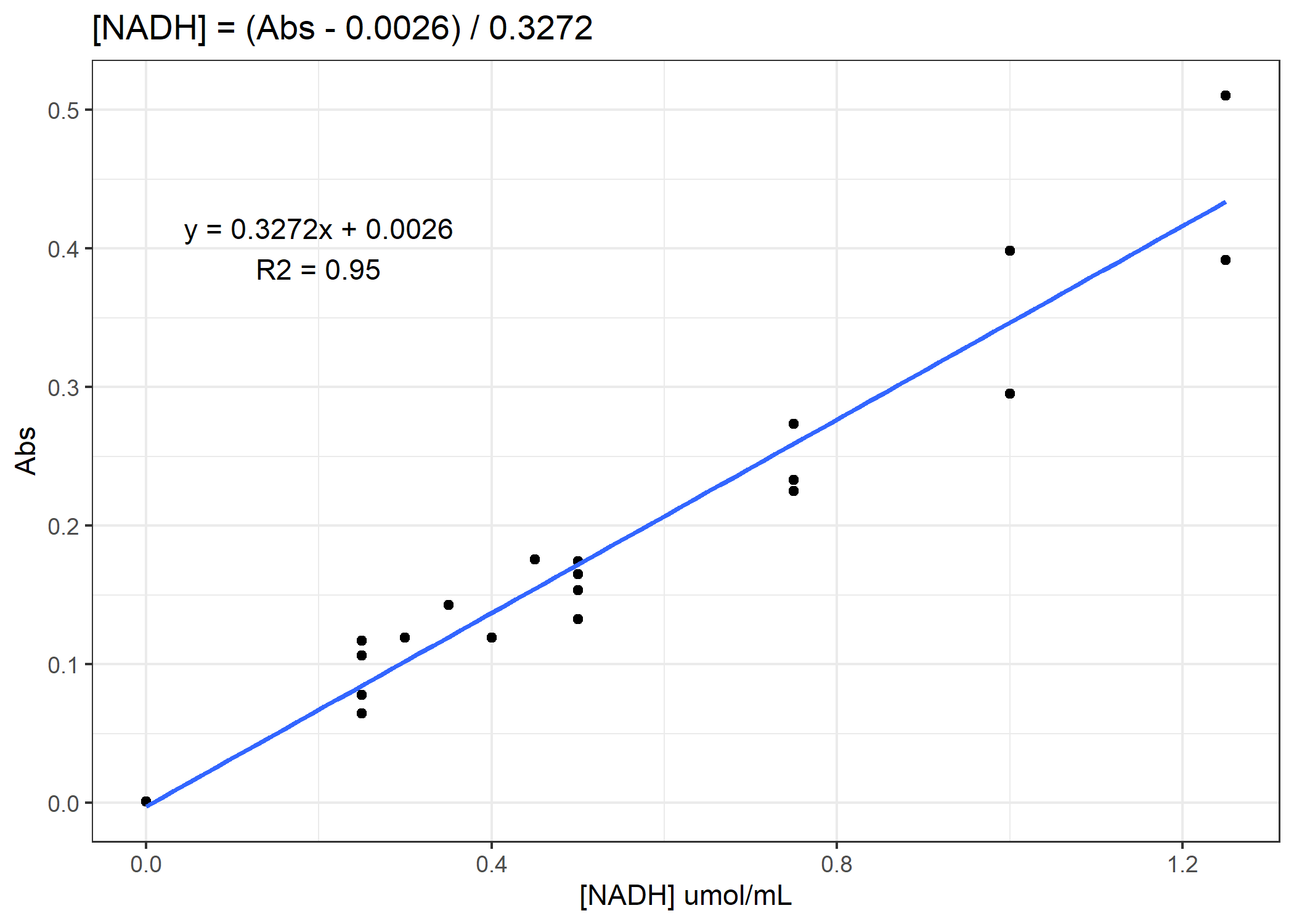
Now we need to convert from our absorbance to our total protein or [NADH] concentration. To do that, we will need to use our standard curves.
Figure 1. Example standard curve for total protein concentration
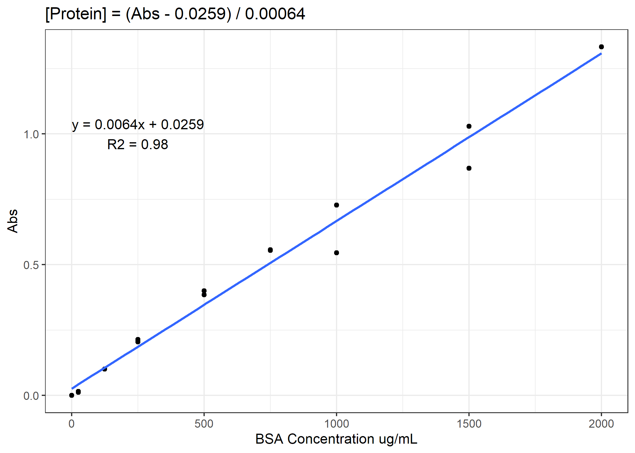
Figure 2. Example standard curve for NADH concentration
Processing Code
See if you can finish the code. You need to calculate total protein and NADH enzyme activity rates for the 4 anaerobic enzymes. For the activity rates, calculate a slope of decomposition over the 30 minutes and standardize this slope to the total protein for that coral sample. Do not forget to subtract out the average of the standard curve 0-points from the total protein samples prior to converting to ug/mL. On average, you need to subtract 0.11 Abs units.
Getting Fancy with Error Propagation
There is uncertainty in everything we measure. Often, we want to calculate this uncertainty and report with our final results. This can get complicated since we have multiple sources of uncertainties and need to figure out the best way to aggregate all sources of error including, the slope of the standard curve and the standard error of the three measurements we took. There may be other independent sources of error, but we’ll just focus on these two for now as an example.
A commonly used technique to solve this problem is called Monte Carlo Error Propagation. Although it has a fancy sounding name, it’s actually quite simple and can be accomplished in only a few lines of code. You can read more online about Monte Carlo Error Propagation, but the basic set of assumptions is that the standard deviation we calculated for our data closely approximates the population standard deviation of the measurement, which would be calculated by taking an infinite number of measurements of the sample. The population standard deviation, therefore, can be estimated by taking randomly selected points, within a normal or Gaussian distribution, and propagating our errors accordingly.
First, multiply the standard deviation you calculated by 1,000 randomly distributed normal numbers using the rnorm function. Then add these standard deviations to the value you calculated. Do this for each term in the value you are calculating. Finally, take the mean of these 1,000 values and use as your accepted value, and then take the standard deviation of these 1,000 numbers as the error propagated standard error. It sounds confusing in words, but take a look at the code below and think about what each of the terms are doing.
Where might this be useful? Well here, you combined the errors from replicate protein aliquots and the errors associated with the standard curve to estimate the total uncertainties of the protein content in the coral you sampled. In the future, perhaps you create a complex equation that models how sea level rise will change in the future. There are uncertainties in the present sea level you measure, plus the thermal expansion term, the projected heating rate, the effect of gravity, and so forth… The deeper you get into science, the more measurements you take and the more uncertainties that exist with each measurement. Monte Carlo Error Propagation is an easy way to quantify the uncertainty with your final estimate.
#define the se of the m term from the standard curve
m_err <- 2.309e-05

mcExample <- mcExample %>%
  mutate(protein.normal = ((Abs-0.11)-0.0259)/0.0006,
         protein.mc = mean((((Abs-0.11)+rnorm(1000)*sd)-0.0259)/(0.0006+rnorm(1000)*m_err)),
         protein.mc_err = sd((((Abs-0.11)+rnorm(1000)*sd)-0.0259)/(0.0006+rnorm(1000)*m_err)))
Table 4. Example of error propagation
| sample | type | Abs | sd | protein.normal | protein.mc | protein.mc_err |
|---|---|---|---|---|---|---|
| D1 | PROTEIN | 0.3718667 | 0.0055429 | 393.2778 | 394.0480 | 17.13507 |
| D10 | PROTEIN | 0.5114333 | 0.0236673 | 625.8889 | 627.0584 | 45.90802 |
| D11 | PROTEIN | 0.5755000 | 0.0165176 | 732.6667 | 734.9354 | 40.31092 |
| D12 | PROTEIN | 0.4844667 | 0.0077106 | 580.9444 | 584.1126 | 26.88848 |
| D2 | PROTEIN | 0.4010333 | 0.0071009 | 441.8889 | 442.0999 | 20.32946 |
You can see there is only a slight difference in the accepted value using the standard calculation or the Monte Carlo calculation. This is due to the 1000 random points selected within a random distribution of the associated error. Since these points are random, each time you rerun the code (unless you set a seed), you will calculate a slightly different value. These values, however, will be well within the associated error calculated in the last column.